前言
对于图的算法,在图的不同表示结构下(例如邻接表和邻接矩阵)有不同的具体实现方式,但是具体的算法思路是一致的,因而在学习过程中只需要掌握好一种结构下的具体实现,在面对其它结构时,将其结构调整到我们所熟悉的那一种就能够搞定它。
本part中的算法均使用以下图结构实现:
Node节点结构:
1
2
3
4
5
6
7
8
9
10
11
12
13
14
15
16
17
18
19
20
21
22
23
24
| package p6.graph;
import java.util.ArrayList;
public class Node {
public int value;
public int in;
public int out;
public ArrayList<Node> nexts;
public ArrayList<Edge> edges;
public Node(int value){
this.value = value;
in = 0;
out = 0;
nexts = new ArrayList<>();
edges = new ArrayList<>();
}
}
|
Edge边结构:
1
2
3
4
5
6
7
8
9
10
11
12
13
14
15
16
17
18
| package p6.graph;
public class Edge {
public int weight;
public Node from;
public Node to;
public Edge(int weight, Node from, Node to){
this.weight = weight;
this.from = from;
this.to = to;
}
}
|
Graph图结构:
1
2
3
4
5
6
7
8
9
10
11
12
13
14
15
16
17
18
| package p6.graph;
import java.util.HashMap;
import java.util.HashSet;
public class Graph {
public HashMap<Integer, Node> nodes;
public HashSet<Edge> edges;
public Graph(){
nodes = new HashMap<>();
edges = new HashSet<>();
}
}
|
图的遍历
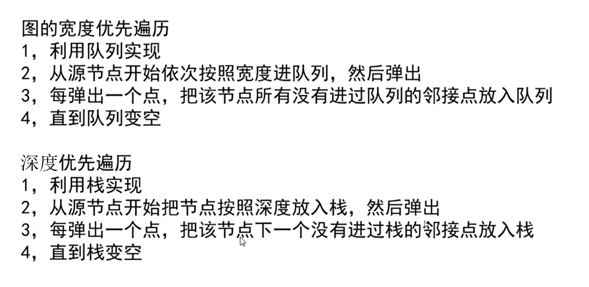
对于如下图,其BFS序列为[A, B, C, D, E,
F],其中,同一层次的遍历顺序不分先后(例如,也可以为[A, B, D, C, E,
F])
DFS序列为[A, B, E, C, F,
D],与BFS相同,DFS序列也能够存在多个不同序列

图的BFS↓
1
2
3
4
5
6
7
8
9
10
11
12
13
14
15
16
17
18
19
20
21
22
23
24
25
26
27
28
29
30
31
32
33
| package p6.graph;
import java.util.HashSet;
import java.util.LinkedList;
import java.util.Queue;
import java.util.Set;
public class GraphBfs {
public void graphBfs(Node node){
if(node == null) return;
Set<Node> set = new HashSet<>();
Queue<Node> queue = new LinkedList<>();
set.add(node);
queue.offer(node);
while(!queue.isEmpty()){
node = queue.poll();
System.out.println(node.value);
for (Node temp : node.nexts) {
if(!set.contains(temp)){
set.add(temp);
queue.offer(temp);
}
}
}
}
}
|
以set存储节点并逐一比对,便于区分图中是否有环
图的DFS↓
1
2
3
4
5
6
7
8
9
10
11
12
13
14
15
16
17
18
19
20
21
22
23
24
25
26
27
28
29
30
31
32
33
| package p6.graph;
import java.util.*;
public class Code02_GraphDFS {
public void graphDfs(Node node){
if(node == null) return;
Set<Node> set = new HashSet<>();
Stack<Node> stack = new Stack<>();
set.add(node);
stack.push(node);
System.out.println(node.value);
while(!stack.isEmpty()){
node = stack.pop();
for (Node temp : node.nexts) {
if(!set.contains(temp)){
stack.push(temp);
set.add(temp);
System.out.println(temp.value);
stack.push(node);
break;
}
}
}
}
}
|
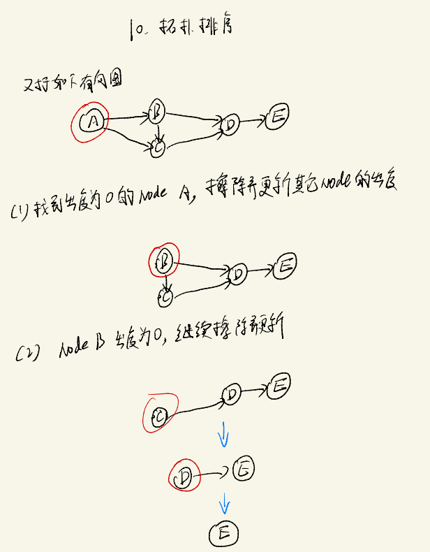
拓扑排序算法
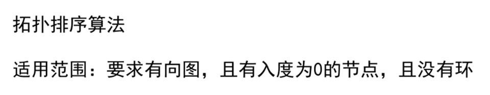
拓扑排序仅适用于无环图
拓扑排序常用于有依赖项的应用中,例如对于一个工程,工程B完成后,才能开始A工程,那么应当保证工程的正确执行顺序以避免阻塞,拓扑排序算法思路如下:
1
2
3
4
5
6
7
8
9
10
11
12
13
14
15
16
17
18
19
20
21
22
23
24
25
26
27
28
29
30
31
32
33
34
35
36
37
38
39
40
41
42
43
| package p6.graph;
import java.util.*;
public class Code03_TopoSort {
public ArrayList<Node> topoSort(Graph graph){
if(graph == null) return null;
Map<Node, Integer> map = new HashMap<>();
Queue<Node> queue = new LinkedList<>();
for (Node node : graph.nodes.values()) {
map.put(node, node.out);
if(node.out == 0){
queue.offer(node);
}
}
ArrayList<Node> res = new ArrayList<>();
while(!queue.isEmpty()){
Node temp = queue.poll();
res.add(temp);
for (Node next : temp.nexts) {
map.put(next, map.get(next) - 1);
if(map.get(next) == 0){
queue.offer(next);
}
}
}
return res;
}
}
|
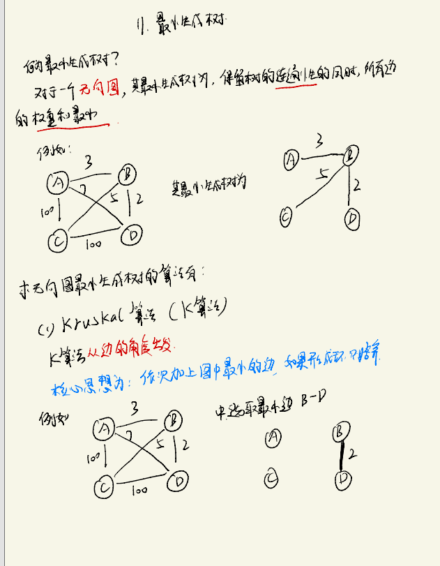
最小生成树
求最小生成树的算法有Kruskal算法和Prim算法,两种算法均用于无向图中,区别在于K算法以边为参考,而P算法以点为参考
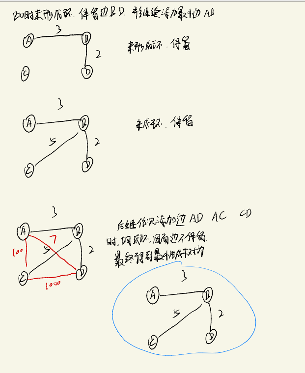
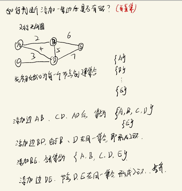
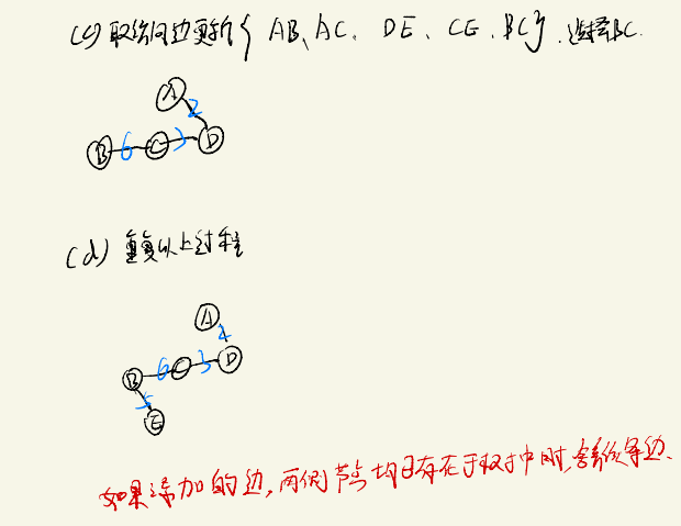
Kruskal算法
算法思路如下:
实现:
1
2
3
4
5
6
7
8
9
10
11
12
13
14
15
16
17
18
19
20
21
22
23
24
25
26
27
28
29
30
31
32
33
34
35
36
37
38
39
40
41
42
43
44
45
46
47
48
49
50
51
52
53
54
55
56
57
58
59
60
61
62
63
64
65
66
67
68
69
70
71
| package p6.graph;
import java.util.*;
public class Code04_Kruskal {
public Map<Node, Set<Node>> mySet(Graph graph){
if(graph == null) return null;
Map<Node, Set<Node>> map = new HashMap<>();
for (Node node : graph.nodes.values()) {
Set<Node> set = new HashSet<>();
set.add(node);
map.put(node, set);
}
return map;
}
public boolean isSameSet(Map<Node, Set<Node>> map, Node A, Node B){
return map.get(A) == map.get(B);
}
public void union(Map<Node, Set<Node>> map, Node A, Node B){
Set<Node> fromSet = map.get(A);
Set<Node> toSet = map.get(B);
for (Node node : toSet) {
if(!fromSet.contains(node)){
fromSet.add(node);
}
}
map.put(B, fromSet);
}
public class myComparator implements Comparator<Edge>{
@Override
public int compare(Edge o1, Edge o2) {
return o1.weight - o2.weight;
}
}
public Set<Edge> kruskal(Graph graph){
if(graph == null) return null;
Map<Node, Set<Node>> map = mySet(graph);
Set<Edge> res = new HashSet<>();
PriorityQueue<Edge> queue = new PriorityQueue<>(new myComparator());
for (Edge edge : graph.edges) {
queue.add(edge);
}
while (!queue.isEmpty()){
Edge edge = queue.poll();
if(!isSameSet(map, edge.from, edge.to)){
res.add(edge);
union(map, edge.from, edge.to);
}
}
return res;
}
}
|
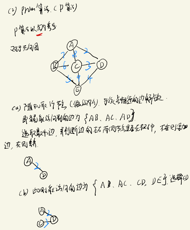
Prim算法
算法思路如下:
实现:
1
2
3
4
5
6
7
8
9
10
11
12
13
14
15
16
17
18
19
20
21
22
23
24
25
26
27
28
29
30
31
32
33
34
35
36
37
38
39
40
41
42
43
44
45
46
47
48
49
50
51
52
53
54
55
| package p6.graph;
import java.util.Comparator;
import java.util.HashSet;
import java.util.PriorityQueue;
import java.util.Set;
public class Code05_Prim {
public class myComparator implements Comparator<Edge>{
@Override
public int compare(Edge o1, Edge o2) {
return o1.weight - o2.weight;
}
}
public Set<Edge> prim(Graph graph){
if(graph == null) return null;
Set<Node> set = new HashSet<>();
PriorityQueue<Edge> queue = new PriorityQueue<>(new myComparator());
Set<Edge> res = new HashSet<>();
for (Node node : graph.nodes.values()) {
if(!set.contains(node)){
set.add(node);
for (Edge edge : node.edges) {
queue.add(edge);
}
while(!queue.isEmpty()){
Edge edge = queue.poll();
if(!set.contains(edge.to)){
res.add(edge);
set.add(edge.to);
for (Edge temp : edge.to.edges) {
queue.offer(temp);
}
}
}
}
}
return res;
}
}
|
prim函数中的for循环是为了防止出现无连通图,对其中的森林进行处理,逐一生成最小生成树
最短路径
求两个节点之间的最短路径,利用Dijkstra算法和Floyd算法求解
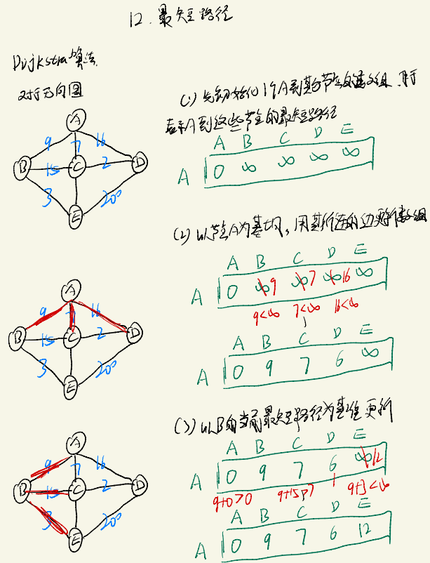
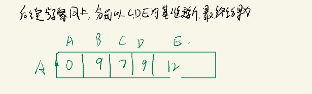
Dijkstra算法
Dijkstra算法适用于没有负数权值边(可以有累加值为负数的边,但不能有累加值为负数的环)的图,给定一个起始节点,求该起始节点到所有节点的最小路径
其算法思想如↓
实现:
1
2
3
4
5
6
7
8
9
10
11
12
13
14
15
16
17
18
19
20
21
22
23
24
25
26
27
28
29
30
31
32
33
34
35
36
37
38
39
40
41
42
43
44
45
46
47
48
49
50
51
52
53
54
55
56
57
| package p6.graph;
import java.util.HashMap;
import java.util.HashSet;
import java.util.Map;
public class Code06_Dijkstra {
public HashMap<Node, Integer> dijkstra(Node head){
if(head == null) return null;
HashMap<Node, Integer> map = new HashMap<>();
map.put(head, 0);
HashSet<Node> selectedSet = new HashSet<>();
Node minNode = getMinEdgeAndNoSelectedNode(map, selectedSet);
while(minNode != null){
int distance = map.get(minNode);
for (Edge edge : minNode.edges) {
Node toNode = edge.to;
if(!map.containsKey(toNode)){
map.put(toNode, distance + edge.weight);
}else{
map.put(toNode, Math.min(map.get(toNode), distance + edge.weight));
}
}
selectedSet.add(minNode);
minNode = getMinEdgeAndNoSelectedNode(map, selectedSet);
}
return map;
}
private Node getMinEdgeAndNoSelectedNode(HashMap<Node, Integer> map, HashSet<Node> selectedSet) {
Node minNode = null;
int minDistance = Integer.MAX_VALUE;
for (Map.Entry<Node, Integer> entry : map.entrySet()) {
Node temp = entry.getKey();
if(map.get(temp) < minNode.value && selectedSet.contains(temp)){
minNode = temp;
minDistance = map.get(temp);
}
}
return minNode;
}
}
|
总结
该part中详细介绍了图结构的使用,以及常见的图相关算法,其中较为关键的是要能够熟练掌握一种自己所熟悉图结构下算法的具体实现,并能够将其它图结构转化为自己所熟悉的结构